

We have been speaking about blocking in experiments at school at this time, and a pupil requested, “When ought to now we have unequal numbers of items within the therapy and management teams?”
I replied that the best instance is when the therapy is dear. You would have 10,000 individuals in your inhabitants however solely sufficient price range to use the therapy to 100 individuals, so 99% will probably be within the management group. In different settings, the therapy is likely to be disruptive, and, once more, you’d solely apply it to a small fraction of the obtainable items.
However even when value isn’t a priority, and also you simply need to maximize statistical effectivity, it may make sense to assign completely different numbers of items to the 2 teams.
For instance, I began to say, suppose that your outcomes are rather more variable below the therapy than the management. Then to attenuate the fundamental estimate of the therapy impact—the common final result within the therapy group, minus the common among the many controls—you’ll need extra therapy observations, to account for the upper variance.
However then I paused. I used to be struck by confusion.
There are two intuitions right here, and so they go in reverse instructions:
(1) Therapy observations are extra variable than controls. So that you want extra therapy measurements, in order to get a exact sufficient estimate for the therapy group.
(2) Therapy observations are extra variable than controls. So therapy observations are crappier, and you need to commit extra of your price range to the high-quality management measurements.
I had a sense that the right reasoning was (1), not (2), however I wasn’t certain.
So how did I clear up the issue?
Brute drive.
Right here’s the R:
n <- 100
expt_sim <- perform(n, p=0.5, s_c=1, s_t=2){
  n_c <- spherical((1-p)*n)
  n_t <- spherical(p*n)
  se_dif <- sqrt(s_c^2/n_c + s_t^2/n_t)
  se_dif
}
curve(expt_sim(100, x), from=.01, to=.99,
  xlab="Proportion of knowledge within the therapy group",
  ylab="se of estimated therapy impact",
  principal="Assuming sd of measurements isntwice as excessive for handled as for controls",
  bty="l")
And here is the end result:
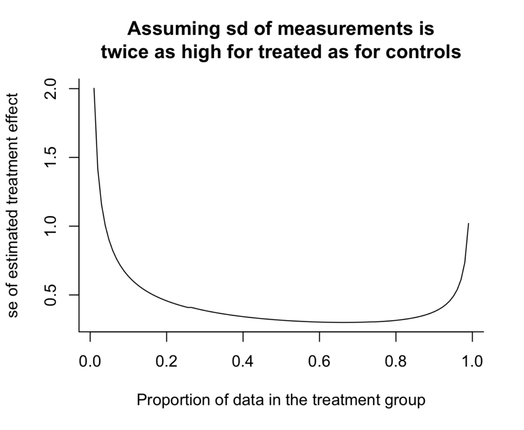
Oh, shoot, I actually do not like how the y-axis would not go all the way in which to zero. It makes the variance discount look extra dramatic than it truly is. Zero is within the neighborhood, so let’s invite it in:
curve(expt_sim(100, x), from=.01, to=.99,
  xlab="Proportion of knowledge within the therapy group",
  ylab="se of estimated therapy impact",
  principal="Assuming sd of measurements isntwice as excessive for handled as for controls",
  bty="l",
  xlim=c(0, 1), ylim=c(0, 2), xaxs="i", yaxs="i")

And we are able to see the reply: if there’s twice as a lot variation within the therapy group as within the management group, then you need to take twice as many measurements within the therapy group. The curve is minimized at x=2/3 (which we may test with out plotting something, however the graph offers some instinct and a sanity test). Argument (1) above is right.
Then again, the usual error from the optimum design is not a lot decrease than the easy 50/50 design, as may be seen by computing the ratio:
print(expt_sim(100, 1/2) / expt_sim(100, 2/3))
which yields 0.95.
Thus, the higher design yields a 5% discount in commonplace error–that is, a ten% effectivity achieve. Not nothing, however not big.
Anyway, the principle level of this submit is you possibly can be taught rather a lot from simulation. After all on this case the issue may be solved analytically—just differentiate (s_c^2/(1-p) + s_t^2/p) with respect to p and set the spinoff to zero, and also you get s_c^2/(1-p)^2 – s_t^2/p^2 = 0, thus s_c^2/(1-p)^2 = s_t^2/p^2, so p/(1-p) = s_t/s_c. That is all superb, however I just like the brute-force answer.


