
In our earlier tutorial, you discovered about RDDs and noticed how Spark’s distributed processing makes large information evaluation attainable. You labored with transformations, actions, and skilled lazy analysis throughout clusters of machines.
However as highly effective as RDDs are, they require you to do a whole lot of handbook work: parsing strings, managing information varieties, writing customized lambda features for each operation, and constructing transformation logic line by line. Whenever you’re constructing information pipelines or working with structured datasets, you will normally need a way more environment friendly and intuitive method.
Spark DataFrames are the answer to this handbook overhead. They supply a higher-level API that handles information parsing, sort administration, and customary operations mechanically. Consider them as pandas DataFrames designed for distributed computing. They allow you to discover and manipulate structured information utilizing acquainted operations like filtering, choosing, grouping, and aggregating, whereas Spark handles the optimization and execution particulars behind the scenes.
Not like RDDs, DataFrames perceive the schema of your information. They know column names, information varieties, and relationships, which implies you’ll be able to write cleaner, extra expressive code, and Spark can optimize it mechanically utilizing its built-in Catalyst optimizer.
To show these ideas, we’ll work with a real-world dataset from the 2010 U.S. Census containing demographic data by age group. This sort of structured information processing represents precisely the form of work the place DataFrames excel: reworking uncooked information into insights with clear, readable code.
By the tip of this tutorial, you’ll:
- Create DataFrames from JSON recordsdata and perceive their construction
- Discover and remodel columns utilizing expressive DataFrame syntax
- Filter rows and compute highly effective aggregations
- Chain operations to construct full information processing pipelines
- Convert DataFrames between PySpark and pandas for visualization
- Perceive when DataFrames provide benefits over RDDs for structured information work
Let’s examine what makes DataFrames Spark’s strongest information abstraction for working with structured data.
Why DataFrames Matter for Information Engineers
DataFrames have grow to be the popular alternative for many Spark purposes, particularly in manufacturing environments. Here is why they’re so precious.
Computerized Optimization with Catalyst
Whenever you write DataFrame operations, Spark’s Catalyst optimizer analyzes your code and creates an optimized execution plan. Not like RDDs the place you are answerable for efficiency optimization, DataFrames mechanically apply strategies like:
- Predicate pushdown: Transferring filters as early as attainable within the processing pipeline
- Column pruning: Studying solely the columns you really want
- Be part of optimization: Selecting essentially the most environment friendly be part of technique based mostly on information dimension and distribution
This implies your DataFrame code usually runs sooner than equal RDD operations, even when the RDD code is well-optimized.
Schema Validation and Information High quality
DataFrames present schema consciousness, which means they mechanically detect and implement the construction of your information, together with column names, information varieties, and constraints. This brings a number of manufacturing benefits:
- Early error detection: Sort mismatches and lacking columns are caught at execution time
- Constant information contracts: Your pipelines can depend on anticipated column names and kinds
- Higher debugging: Schema data helps you perceive information construction points rapidly
That is significantly precious when constructing ETL pipelines that have to deal with altering information sources or implement information high quality requirements.
Acquainted Pandas-like and SQL-like Operations
DataFrames present an API that feels pure whether or not you are coming from pandas or SQL background:
# Pandas-style operations you may know:
# df[df['age'] > 21]                    # filtering
# df[['age', 'total']]                  # choosing columns
# df.groupby('age').depend()             # grouping

# Equal Spark DataFrame operations:
df.filter(df.age > 21)                  # filtering
df.choose("age", "whole")               # choosing columns
df.groupBy("age").depend()               # grouping
This familiarity makes DataFrame code extra readable and maintainable, particularly for groups with blended backgrounds.
Integration with the Broader Spark Ecosystem
DataFrames combine naturally with different Spark parts:
- Spark SQL: Write SQL queries straight in opposition to DataFrames
- MLlib: Machine studying algorithms work natively with DataFrame inputs
- Structured Streaming: Course of real-time information utilizing the identical DataFrame API
Whereas DataFrames provide compelling benefits, RDDs nonetheless have their place. Whenever you want fine-grained management over information distribution, customized algorithms, or processing of unstructured information, RDDs present the flexibleness you want. However for structured information processing—which represents the vast majority of manufacturing workloads—DataFrames provide a extra highly effective and maintainable method.
Exploring Uncooked Information First
Earlier than we begin loading information into DataFrames, let’s check out what we’re working with. Understanding your uncooked information construction is at all times an excellent first step in any information venture.
We’ll be utilizing a dataset from the 2010 U.S. Census that incorporates inhabitants counts damaged down by age and gender. You may obtain this dataset domestically to observe together with the code.
Let’s study the uncooked JSON file construction first:
# Open and study the uncooked file
with open('census_2010.json') as f:
    for i in vary(4):
        print(f.readline(), finish="")
{"females": 1994141, "whole": 4079669, "males": 2085528, "age": 0, "yr": 2010}
{"females": 1997991, "whole": 4085341, "males": 2087350, "age": 1, "yr": 2010}
{"females": 2000746, "whole": 4089295, "males": 2088549, "age": 2, "yr": 2010}
{"females": 2002756, "whole": 4092221, "males": 2089465, "age": 3, "yr": 2010}
This provides us precious insights into our information construction:
- Every line is a legitimate JSON object (not an array of objects)
- Each document has the identical 5 fields:
females,whole,males,age, andyr - All values look like integers
- The information represents particular person age teams from the 2010 Census
With RDDs, you’d have to deal with this parsing manually: studying every line, parsing the JSON, changing information varieties, and coping with any inconsistencies. DataFrames will deal with all of this mechanically, however seeing the uncooked construction first helps us recognize what’s occurring behind the scenes.
From JSON to DataFrames
Now let’s examine how a lot easier the DataFrame method is in comparison with handbook parsing.
Setting Up and Loading Information
import os
import sys
from pyspark.sql import SparkSession

# Guarantee PySpark makes use of the identical Python interpreter
os.environ["PYSPARK_PYTHON"] = sys.executable

# Create SparkSession
spark = SparkSession.builder
    .appName("CensusDataAnalysis")
    .grasp("native[*]")
    .getOrCreate()

# Load JSON straight right into a DataFrame
df = spark.learn.json("census_2010.json")

# Preview the info
df.present(4)
+---+-------+-------+-------+----+
|age|females| males| whole|yr|
+---+-------+-------+-------+----+
| 0|1994141|2085528|4079669|2010|
| 1|1997991|2087350|4085341|2010|
| 2|2000746|2088549|4089295|2010|
| 3|2002756|2089465|4092221|2010|
+---+-------+-------+-------+----+
solely displaying high 4 rowsThat is it! With simply spark.learn.json(), we have achieved what would take dozens of strains of RDD code. Spark mechanically:
- Parsed every JSON line
- Inferred column names from the JSON keys
- Decided acceptable information varieties for every column
- Created a structured DataFrame prepared for evaluation
The .present() technique shows the info in a clear, tabular format that is a lot simpler to learn than uncooked JSON.
Understanding DataFrame Construction and Schema
Considered one of DataFrame’s greatest benefits is computerized schema detection. Consider a schema as a blueprint that tells Spark precisely what your information appears like. Similar to how a blueprint helps architects perceive a constructing’s construction, a schema helps Spark perceive your information’s construction.
Exploring the Inferred Schema
Let’s study what Spark found about our census information:
# Show the inferred schema
df.printSchema()
root
|-- age: lengthy (nullable = true)
|-- females: lengthy (nullable = true)
|-- males: lengthy (nullable = true)
|-- whole: lengthy (nullable = true)
|-- yr: lengthy (nullable = true)This schema tells us a number of necessary issues:
- All columns include
lengthyintegers (excellent for inhabitants counts) - All columns are
nullable = true(can include lacking values) - Column names match our JSON keys precisely
- Spark mechanically selected acceptable information varieties
We will additionally examine the schema programmatically:
# Get column names and information varieties for additional inspection
column_names = df.columns
column_types = df.dtypes

print("Column names:", column_names)
print("Column varieties:", column_types)
Column names: ['age', 'females', 'males', 'total', 'year']
Column varieties: [('age', 'bigint'), ('females', 'bigint'), ('males', 'bigint'), ('total', 'bigint'), ('year', 'bigint')]Why Schema Consciousness Issues
This computerized schema detection supplies speedy advantages:
- Efficiency: Spark can optimize operations as a result of it is aware of information varieties prematurely
- Error Prevention: Sort mismatches are caught early moderately than producing mistaken outcomes
- Code Readability: You may reference columns by identify moderately than by place
- Documentation: The schema serves as residing documentation of your information construction
Examine this to RDDs, the place you’d want to keep up sort data manually and deal with schema validation your self. DataFrames make this easy whereas offering higher efficiency and error checking.
Core DataFrame Operations
Now that we perceive DataFrames and have our census information loaded, let’s discover the core operations you will use in most information processing workflows.
Choosing Columns
Column choice is without doubt one of the most elementary DataFrame operations. The .choose() technique permits you to give attention to particular attributes:
# Choose particular columns for evaluation
age_gender_df = df.choose("age", "males", "females")
age_gender_df.present(10)
+---+-------+-------+
|age| males|females|
+---+-------+-------+
| 0|2085528|1994141|
| 1|2087350|1997991|
| 2|2088549|2000746|
| 3|2089465|2002756|
| 4|2090436|2004366|
| 5|2091803|2005925|
| 6|2093905|2007781|
| 7|2097080|2010281|
| 8|2101670|2013771|
| 9|2108014|2018603|
+---+-------+-------+
solely displaying high 10 rowsDiscover that .choose() returns a brand new DataFrame with solely the desired columns. That is helpful for:
- Decreasing information dimension earlier than executing costly operations
- Getting ready particular column units for various analytical functions
- Creating centered views of your information for workforce members
Creating New Columns
DataFrames excel at creating calculated fields. The .withColumn() technique permits you to add new columns based mostly on current information:
from pyspark.sql.features import col

# Calculate female-to-male ratio
df_with_ratio = df.withColumn("female_male_ratio", col("females") / col("males"))

# Present the improved dataset
ratio_preview = df_with_ratio.choose("age", "females", "males", "female_male_ratio")
ratio_preview.present(10)
+---+-------+-------+------------------+
|age|females| males| female_male_ratio|
+---+-------+-------+------------------+
| 0|1994141|2085528|0.9561804013180355|
| 1|1997991|2087350|0.9571902172611205|
| 2|2000746|2088549|0.9579598084603234|
| 3|2002756|2089465|0.9585018174508786|
| 4|2004366|2090436|0.9588267710659403|
| 5|2005925|2091803|0.9589454647497876|
| 6|2007781|2093905|0.9588691941611487|
| 7|2010281|2097080|0.9586095904781887|
| 8|2013771|2101670| 0.958176592899932|
| 9|2018603|2108014|0.9575851963032503|
+---+-------+-------+------------------+
solely displaying high 10 rowsThe information reveals that the female-to-male ratio is constantly beneath 1.0 for youthful age teams, which means there are barely extra males than females born every year. It is a well-documented demographic phenomenon.
Filtering Rows
DataFrame filters are each extra readable and higher optimized than RDD equivalents. Let’s discover age teams the place males outnumber females:
# Filter rows the place female-to-male ratio is lower than 1
male_dominated_df = df_with_ratio.filter(col("female_male_ratio") < 1)
male_dominated_preview = male_dominated_df.choose("age", "females", "males", "female_male_ratio")
male_dominated_preview.present(5)
+---+-------+-------+------------------+
|age|females| males| female_male_ratio|
+---+-------+-------+------------------+
| 0|1994141|2085528|0.9561804013180355|
| 1|1997991|2087350|0.9571902172611205|
| 2|2000746|2088549|0.9579598084603234|
| 3|2002756|2089465|0.9585018174508786|
| 4|2004366|2090436|0.9588267710659403|
+---+-------+-------+------------------+
solely displaying high 5 rowsThese filtering patterns are frequent in information processing workflows the place it’s good to isolate particular subsets of knowledge based mostly on enterprise logic or analytical necessities.
Aggregations for Abstract Evaluation
Aggregation operations are the place DataFrames actually shine in comparison with RDDs. They supply SQL-like grouping and summarization with computerized optimization.
Primary Aggregations
Let’s begin with easy aggregations throughout your entire dataset:
from pyspark.sql.features import sum

# Calculate whole inhabitants by yr (since all information is from 2010)
total_by_year = df.groupBy("yr").agg(sum("whole").alias("total_population"))
total_by_year.present()
+----+----------------+
|yr|total_population|
+----+----------------+
|2010| 312247116|
+----+----------------+This provides us the whole U.S. inhabitants for 2010 (~312 million), which matches historic Census figures and validates our dataset’s accuracy.
Extra Advanced Aggregations
We will create extra subtle aggregations by grouping information into classes. Let’s discover completely different age ranges:
from pyspark.sql.features import when, avg, depend

# Create age classes and analyze patterns
categorized_df = df.withColumn(
    "age_category",
    when(col("age") < 18, "Baby")
    .when(col("age") < 65, "Grownup")
    .in any other case("Senior")
)

# Group by class and calculate a number of statistics
category_stats = categorized_df.groupBy("age_category").agg(
    sum("whole").alias("total_population"),
    avg("whole").alias("avg_per_age_group"),
    depend("age").alias("age_groups_count")
)

category_stats.present()
+------------+---------------+------------------+----------------+
|age_category|total_population|avg_per_age_group|age_groups_count|
+------------+---------------+------------------+----------------+
| Baby| 74181467| 4121192.6111111 | 18|
| Grownup| 201292894| 4281124.9574468 | 47|
| Senior| 36996966| 1027693.5 | 36|
+------------+---------------+------------------+----------------+This breakdown reveals necessary demographic insights:
- Adults (18-64) characterize the biggest inhabitants section (~201M)
- Youngsters (0-17) have the very best common per age group, displaying larger beginning charges lately
- Seniors (65+) have a lot smaller age teams on common, reflecting historic demographics
Chaining Operations for Advanced Evaluation
Considered one of DataFrame’s biggest strengths is the power to chain operations into readable, maintainable information processing pipelines.
Constructing Analytical Pipelines
Let’s construct an entire analytical workflow that transforms our uncooked census information into insights:
# Chain a number of operations collectively for youngster demographics evaluation
filtered_summary = (
    df.withColumn("female_male_ratio", col("females") / col("males"))
      .withColumn("gender_gap", col("females") - col("males"))
      .filter(col("age") < 18)
      .choose("age", "female_male_ratio", "gender_gap")
)

filtered_summary.present(10)
+---+------------------+----------+
|age| female_male_ratio|gender_gap|
+---+------------------+----------+
| 0|0.9561804013180355| -91387|
| 1|0.9571902172611205| -89359|
| 2|0.9579598084603234| -87803|
| 3|0.9585018174508786| -86709|
| 4|0.9588267710659403| -86070|
| 5|0.9589454647497876| -85878|
| 6|0.9588691941611487| -86124|
| 7|0.9586095904781887| -86799|
| 8| 0.958176592899932| -87899|
| 9|0.9575851963032503| -89411|
+---+------------------+----------+
solely displaying high 10 rowsThis single pipeline performs a number of operations:
- Information enrichment: Calculates gender ratios and gaps
- High quality filtering: Focuses on childhood age teams (below 18)
- Column choice: Returns solely the metrics we’d like for evaluation
The outcomes present that throughout all childhood age teams, there are constantly extra males than females (detrimental gender hole), with the sample being remarkably constant throughout ages.
Efficiency Advantages of DataFrame Chaining
This chained method presents a number of benefits over equal RDD processing:
Computerized Optimization: Spark’s Catalyst optimizer can mix operations, decrease information scanning, and generate environment friendly execution plans for your entire pipeline.
Readable Code: The pipeline reads like an outline of the analytical course of, making it simpler for groups to know and preserve.
Reminiscence Effectivity: Intermediate DataFrames aren’t materialized until explicitly cached, decreasing reminiscence stress.
Examine this to an RDD method, which might require a number of separate transformations, handbook optimization, and way more complicated code to realize the identical outcome.
PySpark DataFrames vs Pandas DataFrames
Now that you have labored with PySpark DataFrames, you is perhaps questioning how they relate to the pandas DataFrames you might already know. Whereas they share many ideas and even some syntax, they’re designed for very completely different use instances.
Key Similarities
Each PySpark and pandas DataFrames share:
- Tabular Construction: Each arrange information in rows and columns with named columns
- Related Operations: Each assist filtering, grouping, choosing, and aggregating information
- Acquainted Syntax: Many operations use related technique names like
.choose(),.filter(), and.groupBy()
Let’s examine their syntax for a typical choose and filter operation:
# PySpark
pyspark_result = df.choose("age", "whole").filter(col("age") > 21)

# Pandas
df_pandas = df.toPandas()  # Convert PySpark df to pandas
pandas_result = df_pandas[df_pandas["age"] > 21][["age", "total"]]

print("PySpark Consequence:")
{pyspark_result.present(5)}
print(f"Pandas Consequence: n{pandas_result[:5]}")
PySpark Consequence:
+---+-------+
|age| whole|
+---+-------+
| 22|4362678|
| 23|4351092|
| 24|4344694|
| 25|4333645|
| 26|4322880|
+---+-------+
solely displaying high 5 rows
Pandas Consequence:
age whole
22 22 4362678
23 23 4351092
24 24 4344694
25 25 4333645
26 26 4322880Key Variations
Nevertheless, there are necessary variations:
- Scale: pandas DataFrames run on a single machine and are restricted by obtainable reminiscence, whereas PySpark DataFrames can course of terabytes of knowledge throughout a number of machines.
- Execution: pandas operations execute instantly, whereas PySpark makes use of lazy analysis and solely executes whenever you name an motion.
- Information Location: pandas masses all information into reminiscence, whereas PySpark can work with information saved throughout distributed methods.
When to Use Every
Use PySpark DataFrames when:
- Working with massive datasets (>5GB)
- Information is saved in distributed methods (HDFS, S3, and so forth.)
- It is advisable to scale processing throughout a number of machines
- Constructing manufacturing information pipelines
Use pandas DataFrames when:
- Working with smaller datasets (<5GB)
- Doing exploratory information evaluation
- Creating visualizations
- Engaged on a single machine
Working Collectively
The actual energy comes from utilizing each collectively. PySpark DataFrames deal with the heavy lifting of processing massive datasets, then you’ll be able to convert outcomes to pandas for visualization and closing evaluation.
Visualizing DataFrame Outcomes
Attributable to PySpark’s distributed nature, you’ll be able to’t straight create visualizations from PySpark DataFrames. The information is perhaps unfold throughout a number of machines, and visualization libraries like matplotlib count on information to be obtainable domestically. The answer is to transform your PySpark DataFrame to a pandas DataFrame first.
Changing PySpark DataFrames to Pandas
Let’s create some visualizations of our census evaluation. First, we’ll put together aggregated information and convert it to pandas:
# Create age group summaries (smaller dataset appropriate for visualization)
age_summary = df.withColumn("female_male_ratio", col("females") / col("males"))
                .choose("age", "whole", "female_male_ratio")
                .filter(col("age") <= 60)

# Convert to pandas DataFrame
age_summary_pandas = age_summary.toPandas()

print("Transformed to pandas:")
print(f"Sort: {sort(age_summary_pandas)}")
print(f"Form: {age_summary_pandas.form}")
print(age_summary_pandas.head())
Transformed to pandas:
Sort:
Form: (61, 3)
age whole female_male_ratio
0 0 4079669 0.956180
1 1 4085341 0.957190
2 2 4089295 0.957960
3 3 4092221 0.958502
4 4 4094802 0.958827 Creating Visualizations
Now we will create visualizations utilizing matplotlib:
import matplotlib.pyplot as plt

# Create visualizations
fig, (ax1, ax2) = plt.subplots(1, 2, figsize=(15, 6))

# Plot 1: Inhabitants by age
ax1.plot(age_summary_pandas['age'], age_summary_pandas['total'], marker='o')
ax1.set_title('Inhabitants by Age (Ages 0-60)')
ax1.set_xlabel('Age')
ax1.set_ylabel('Complete Inhabitants')
ax1.grid(True)

# Plot 2: Feminine-to-Male Ratio by age
ax2.plot(age_summary_pandas['age'], age_summary_pandas['female_male_ratio'],
         marker='s', colour='crimson')
ax2.axhline(y=1.0, colour='black', linestyle='--', alpha=0.7, label='Equal ratio')
ax2.set_title('Feminine-to-Male Ratio by Age')
ax2.set_xlabel('Age')
ax2.set_ylabel('Feminine-to-Male Ratio')
ax2.legend()
ax2.grid(True)

plt.tight_layout()
plt.present()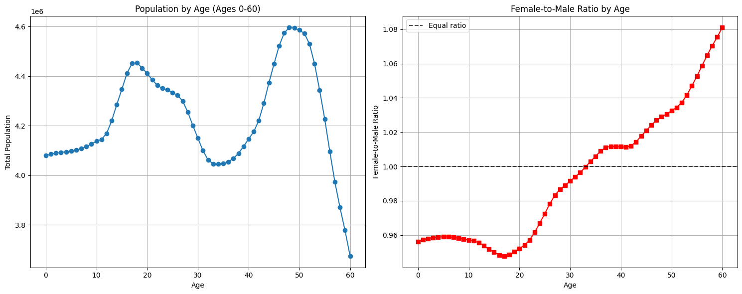
These visualizations reveal demographic patterns that may be troublesome to identify in uncooked numbers:
- Two distinct inhabitants peaks: One round ages 17-18 and one other bigger peak round ages 47-50, doubtless reflecting child increase generations
- Beginning ratio patterns: Extra males are born than females (ratio beneath 1.0 for younger ages), which is a well-documented organic phenomenon
- Ageing demographics: The feminine-to-male ratio crosses 1.0 round age 34 and continues rising, reflecting longer feminine life expectancy
- Era results: The dramatic inhabitants drop after age 50 and the valley round ages 30-35 reveal distinct generational cohorts within the 2010 census information
Essential Concerns for Conversion
When changing PySpark DataFrames to pandas, hold these factors in thoughts:
-
Dimension Limitations: pandas DataFrames should slot in reminiscence on a single machine. All the time filter or mixture your PySpark DataFrame first to cut back dimension.
-
Use Sampling: For very massive datasets, take into account sampling earlier than conversion:
# Pattern of knowledge earlier than changing sample_df = large_df.pattern(fraction=0.1) sample_pandas = sample_df.toPandas() -
Combination First: Create summaries in PySpark, then convert the smaller outcome:
# Combination in PySpark, then convert
abstract = df.groupBy("class").agg(sum("worth").alias("whole"))
summary_pandas = abstract.toPandas()  # A lot smaller than authentic
This workflow—course of large information with PySpark, then convert summaries to pandas for visualization—represents a typical and highly effective sample in information evaluation.
DataFrames vs RDDs: Selecting the Proper Software
After working with each RDDs and DataFrames, you have got a sensible basis for selecting the best device. Here is a choice framework that will help you weigh your choices:
Select DataFrames When:
- Working with structured information: In case your information has a transparent schema with named columns and constant varieties, DataFrames present important benefits in readability and efficiency.
- Constructing ETL pipelines: DataFrames excel on the extract, remodel, and cargo operations frequent in information engineering workflows. Their SQL-like operations and computerized optimization make complicated transformations extra maintainable.
- Crew collaboration: DataFrame operations are extra accessible to workforce members with SQL backgrounds, and the structured nature makes code critiques simpler.
- Efficiency issues: For many structured information operations, DataFrames will outperform equal RDD code as a result of Catalyst optimization.
Select RDDs When:
- Processing unstructured information: When working with uncooked textual content, binary information, or complicated nested constructions that do not match the tabular mannequin.
- Implementing customized algorithms: In case you want fine-grained management over information distribution, partitioning, or customized transformation logic.
- Working with key-value pairs: Some RDD operations like
reduceByKey()andaggregateByKey()present extra direct management over grouped operations. - Most flexibility: When it’s good to implement operations that do not map effectively to DataFrame’s SQL-like paradigm.
A Sensible Instance
Contemplate processing internet server logs. You may begin with RDDs to parse uncooked log strains:
# RDD method for preliminary parsing of unstructured textual content
log_rdd = spark.sparkContext.textFile("server.log")
parsed_rdd = log_rdd.map(parse_log_line).filter(lambda x: x isn't None)
However after getting structured information, swap to DataFrames for evaluation:
# Convert to DataFrame for structured evaluation
log_schema = ["timestamp", "ip", "method", "url", "status", "size"]
log_df = spark.createDataFrame(parsed_rdd, log_schema)

# Use DataFrame operations for evaluation
error_summary = log_df
    .filter(col("standing") >= 400)
    .groupBy("standing", "url")
    .depend()
    .orderBy("depend", ascending=False)
This hybrid method makes use of the strengths of each abstractions: RDD flexibility for parsing and DataFrame optimization for evaluation.
Subsequent Steps and Sources
You’ve got now discovered Spark DataFrames and perceive how they bring about construction, efficiency, and expressiveness to distributed information processing. You’ve got seen how they differ from each RDDs and pandas DataFrames, and also you perceive when to make use of every device.
All through this tutorial, you discovered:
- DataFrame fundamentals: How schema consciousness and computerized optimization make structured information processing extra environment friendly
- Core operations: Choosing, filtering, reworking, and aggregating information utilizing clear, readable syntax
- Pipeline constructing: Chaining operations to create maintainable information processing workflows
- Integration with pandas: Changing between PySpark and pandas DataFrames for visualization
- Software choice: A sensible framework for selecting between DataFrames and RDDs
The DataFrame ideas you have discovered right here kind the inspiration for many fashionable Spark purposes. Whether or not you are constructing ETL pipelines, getting ready information for machine studying, or creating analytical stories, DataFrames present the instruments it’s good to work effectively at scale.
Transferring Ahead
Your subsequent steps within the Spark ecosystem construct naturally on this DataFrame basis:
Spark SQL: Learn to question DataFrames utilizing acquainted SQL syntax, making complicated analytics extra accessible to groups with database backgrounds.
Superior DataFrame Operations: Discover window features, complicated joins, and superior aggregations that deal with subtle analytical necessities.
Efficiency Tuning: Uncover caching methods, partitioning strategies, and optimization approaches that make your DataFrame purposes run sooner in manufacturing.
Hold Studying
For deeper exploration of those ideas, take a look at these sources:
You’ve got taken one other important step in understanding distributed information processing. The mixture of RDD fundamentals and DataFrame expressiveness provides you the flexibleness to deal with large information challenges. Hold experimenting, hold constructing, and most significantly, continue to learn!

