

On this information, I am going to stroll you thru analyzing film ranking information to find out if Fandango’s ranking system modified after being uncovered for potential bias. This guided undertaking, Investigating Fandango Film Scores, will allow you to develop hands-on expertise in information cleansing, exploratory evaluation, and statistical comparability utilizing Python.
We’ll assume the position of an information journalist investigating whether or not Fandango—a film ticket gross sales and scores web site—adjusted its ranking system following a high-profile evaluation in 2015 that recommended it was inflating film scores.
What You may Be taught:
- Find out how to clear and put together datasets for statistical comparability
- Find out how to visualize and interpret ranking distributions
- Find out how to use frequency tables and abstract statistics to disclose information patterns
- How to attract conclusions from information and perceive its limitations
- Find out how to set up your evaluation workflow in a Jupyter Pocket book
Earlier than diving into this undertaking, make sure you’re snug with Python fundamentals, NumPy and pandas library fundamentals, and information visualization with matplotlib. For those who’re new to those ideas, these foundational expertise are lined in Dataquest’s Python Fundamentals for Information Evaluation course.
Now, let’s start our investigation!
Step 1: Setting Up the Setting
For those who’re engaged on this undertaking throughout the Dataquest platform, you’ll be able to skip this step as the whole lot is already arrange for you. Nonetheless, if you would like to work domestically, guarantee you’ve gotten the next arrange:
- Jupyter Pocket book: Set up Jupyter Pocket book or JupyterLab to simply mix code, visualize outcomes, and clearly doc your evaluation utilizing markdown cells as you’re employed by means of this undertaking. Alternatively, use Google Colab for a cloud-based choice that requires no set up.
- Required Libraries: We’ll be utilizing pandas and NumPy for information manipulation and matplotlib for visualization.
- Dataset Information: Obtain the 2 dataset recordsdata from the hyperlinks under:
Now, let’s dive into our evaluation!
Step 2: Understanding the Challenge Background
In October 2015, Walt Hickey, an information journalist at FiveThirtyEight, revealed a compelling evaluation exhibiting that Fandango’s film ranking system seemed to be biased and dishonest. His proof recommended that Fandango was inflating scores, probably to encourage ticket gross sales on their platform (since they promote film tickets along with internet hosting evaluations).
After Hickey’s evaluation went public, Fandango responded by claiming the inflated scores had been brought on by a “bug” of their system that rounded scores as much as the closest half-star. They promised to repair this challenge.
Our objective is to find out whether or not Fandango really modified their ranking system following this controversy by evaluating film scores earlier than and after Hickey’s evaluation.
Step 3: Opening and Exploring the Information
Let’s begin by importing pandas, loading our two datasets, and looking out on the first few rows. We’ll be evaluating film scores from earlier than and after the 2015 evaluation.
import pandas as pd

prior = pd.read_csv('fandango_score_comparison.csv')
after = pd.read_csv('movie_ratings_16_17.csv')

prior.head()| FILM | RottenTomatoes | RottenTomatoes_User | Metacritic | Metacritic_User | IMDB | Fandango_Stars | Fandango_Ratingvalue | RT_norm | RT_user_norm | … | IMDB_norm | RT_norm_round | RT_user_norm_round | Metacritic_norm_round | Metacritic_user_norm_round | IMDB_norm_round | Metacritic_user_vote_count | IMDB_user_vote_count | Fandango_votes | Fandango_Difference | |
|---|---|---|---|---|---|---|---|---|---|---|---|---|---|---|---|---|---|---|---|---|---|
| 0 | Avengers: Age of Ultron (2015) | 74 | 86 | 66 | 7.1 | 7.8 | 5.0 | 4.5 | 3.70 | 4.3 | … | 3.90 | 3.5 | 4.5 | 3.5 | 3.5 | 4.0 | 1330 | 271107 | 14846 | 0.5 |
| 1 | Cinderella (2015) | 85 | 80 | 67 | 7.5 | 7.1 | 5.0 | 4.5 | 4.25 | 4.0 | … | 3.55 | 4.5 | 4.0 | 3.5 | 4.0 | 3.5 | 249 | 65709 | 12640 | 0.5 |
| 2 | Ant-Man (2015) | 80 | 90 | 64 | 8.1 | 7.8 | 5.0 | 4.5 | 4.00 | 4.5 | … | 3.90 | 4.0 | 4.5 | 3.0 | 4.0 | 4.0 | 627 | 103660 | 12055 | 0.5 |
| 3 | Do You Imagine? (2015) | 18 | 84 | 22 | 4.7 | 5.4 | 5.0 | 4.5 | 0.90 | 4.2 | … | 2.70 | 1.0 | 4.0 | 1.0 | 2.5 | 2.5 | 31 | 3136 | 1793 | 0.5 |
| 4 | Scorching Tub Time Machine 2 (2015) | 14 | 28 | 29 | 3.4 | 5.1 | 3.5 | 3.0 | 0.70 | 1.4 | … | 2.55 | 0.5 | 1.5 | 1.5 | 1.5 | 2.5 | 88 | 19560 | 1021 | 0.5 |
| 5 rows × 22 columns | |||||||||||||||||||||
If you run the code above, you will see that the prior dataset accommodates a number of film ranking sources, together with Rotten Tomatoes, Metacritic, IMDB, and Fandango. Earlier than we get to our evaluation, we’ll be certain that we filter this all the way down to solely columns associated to Fandango.
Now let’s take a peek on the after dataset to see the way it compares:
after.head()| film | 12 months | metascore | imdb | tmeter | viewers | fandango | n_metascore | n_imdb | n_tmeter | n_audience | nr_metascore | nr_imdb | nr_tmeter | nr_audience | |
|---|---|---|---|---|---|---|---|---|---|---|---|---|---|---|---|
| 0 | 10 Cloverfield Lane | 2016 | 76 | 7.2 | 90 | 79 | 3.5 | 3.80 | 3.60 | 4.50 | 3.95 | 4.0 | 3.5 | 4.5 | 4.0 |
| 1 | 13 Hours | 2016 | 48 | 7.3 | 50 | 83 | 4.5 | 2.40 | 3.65 | 2.50 | 4.15 | 2.5 | 3.5 | 2.5 | 4.0 |
| 2 | A Treatment for Wellness | 2016 | 47 | 6.6 | 40 | 47 | 3.0 | 2.35 | 3.30 | 2.00 | 2.35 | 2.5 | 3.5 | 2.0 | 2.5 |
| 3 | A Canine’s Function | 2017 | 43 | 5.2 | 33 | 76 | 4.5 | 2.15 | 2.60 | 1.65 | 3.80 | 2.0 | 2.5 | 1.5 | 4.0 |
| 4 | A Hologram for the King | 2016 | 58 | 6.1 | 70 | 57 | 3.0 | 2.90 | 3.05 | 3.50 | 2.85 | 3.0 | 3.0 | 3.5 | 3.0 |
The after dataset additionally accommodates scores from numerous sources, however its construction is barely completely different. The column names and group do not precisely match the prior dataset, which is one thing we’ll want to handle.
Let’s look at the details about every dataset utilizing the DataFrame data() methodology to higher perceive what we’re working with:
    prior.data()


RangeIndex: 146 entries, 0 to 145
Information columns (complete 22 columns):
 #   Column                       Non-Null Depend  Dtype
---  ------                       --------------  -----
 0   FILM                         146 non-null    object
 1   RottenTomatoes               146 non-null    int64
 2   RottenTomatoes_User          146 non-null    int64
 3   Metacritic                   146 non-null    int64
 4   Metacritic_User              146 non-null    float64
 5   IMDB                         146 non-null    float64
 6   Fandango_Stars               146 non-null    float64
 7   Fandango_Ratingvalue         146 non-null    float64
 8   RT_norm                      146 non-null    float64
 9   RT_user_norm                 146 non-null    float64
 10  Metacritic_norm              146 non-null    float64
 11  Metacritic_user_nom          146 non-null    float64
 12  IMDB_norm                    146 non-null    float64
 13  RT_norm_round                146 non-null    float64
 14  RT_user_norm_round           146 non-null    float64
 15  Metacritic_norm_round        146 non-null    float64
 16  Metacritic_user_norm_round   146 non-null    float64
 17  IMDB_norm_round              146 non-null    float64
 18  Metacritic_user_vote_count   146 non-null    int64
 19  IMDB_user_vote_count         146 non-null    int64
 20  Fandango_votes               146 non-null    int64
 21  Fandango_Difference          146 non-null    float64
dtypes: float64(15), int64(6), object(1)
reminiscence utilization: 25.2+ KB
    after.data()


RangeIndex: 214 entries, 0 to 213
Information columns (complete 15 columns):
 #   Column         Non-Null Depend  Dtype
---  ------         --------------  -----
 0   film          214 non-null    object
 1   12 months           214 non-null    int64
 2   metascore      214 non-null    int64
 3   imdb           214 non-null    float64
 4   tmeter         214 non-null    int64
 5   viewers       214 non-null    int64
 6   fandango       214 non-null    float64
 7   n_metascore    214 non-null    float64
 8   n_imdb         214 non-null    float64
 9   n_tmeter       214 non-null    float64
 10  n_audience     214 non-null    float64
 11  nr_metascore   214 non-null    float64
 12  nr_imdb        214 non-null    float64
 13  nr_tmeter      214 non-null    float64
 14  nr_audience    214 non-null    float64
dtypes: float64(10), int64(4), object(1)
reminiscence utilization: 25.2+ KB
As we are able to see, the datasets have completely different column names, constructions, and even completely different numbers of entries—the prior dataset has 146 motion pictures, whereas the after dataset accommodates 214 motion pictures. Earlier than we are able to make a significant comparability, we have to clear and put together our information by focusing solely on the related Fandango scores.
Step 4: Information Cleansing
Since we’re solely inquisitive about Fandango’s scores, let’s create new dataframes utilizing copy() by deciding on simply the columns we’d like for our evaluation:
prior = prior[['FILM',
               'Fandango_Stars',
               'Fandango_Ratingvalue',
               'Fandango_votes',
               'Fandango_Difference']].copy()
after = after[['movie',
               'year',
               'fandango']].copy()

prior.head()
after.head()| FILM | Fandango_Stars | Fandango_Ratingvalue | Fandango_votes | Fandango_Difference | |
|---|---|---|---|---|---|
| 0 | Avengers: Age of Ultron (2015) | 5.0 | 4.5 | 14846 | 0.5 |
| 1 | Cinderella (2015) | 5.0 | 4.5 | 12640 | 0.5 |
| 2 | Ant-Man (2015) | 5.0 | 4.5 | 12055 | 0.5 |
| 3 | Do You Imagine? (2015) | 5.0 | 4.5 | 1793 | 0.5 |
| 4 | Scorching Tub Time Machine 2 (2015) | 3.5 | 3.0 | 1021 | 0.5 |
| film | 12 months | fandango | |
|---|---|---|---|
| 0 | 10 Cloverfield Lane | 2016 | 3.5 |
| 1 | 13 Hours | 2016 | 4.5 |
| 2 | A Treatment for Wellness | 2016 | 3.0 |
| 3 | A Canine’s Function | 2017 | 4.5 |
| 4 | A Hologram for the King | 2016 | 3.0 |
One key distinction is that our prior dataset does not have a devoted ‘12 months’ column, however we are able to see the 12 months is included on the finish of every film title (in parentheses). Let’s extract that data and place it in a brand new ‘12 months’ column:
prior['year'] = prior['FILM'].str[-5:-1]
prior.head()| FILM | Fandango_Stars | Fandango_Ratingvalue | Fandango_votes | Fandango_Difference | Yr | |
|---|---|---|---|---|---|---|
| 0 | Avengers: Age of Ultron (2015) | 5.0 | 4.5 | 14846 | 0.5 | 2015 |
| 1 | Cinderella (2015) | 5.0 | 4.5 | 12640 | 0.5 | 2015 |
| 2 | Ant-Man (2015) | 5.0 | 4.5 | 12055 | 0.5 | 2015 |
| 3 | Do You Imagine? (2015) | 5.0 | 4.5 | 1793 | 0.5 | 2015 |
| 4 | Scorching Tub Time Machine 2 (2015) | 3.5 | 3.0 | 1021 | 0.5 | 2015 |
The code above makes use of string slicing to extract the 12 months from the movie title. By utilizing detrimental indexing ([-5:-1]), we’re taking characters ranging from the fifth-to-last (-5) as much as (however not together with) the final character (-1). This neatly captures the 12 months whereas avoiding the closing parenthesis. If you run this code, you will see that every film now has a corresponding 12 months worth extracted from its title.
Now that we’ve got the 12 months data for each datasets, let’s verify which years are included within the prior dataset utilizing the Collection value_counts() methodology:
prior['year'].value_counts()12 months
2015 129
2014 17
Title: depend, dtype: int64From the output above, we are able to see that the prior dataset contains motion pictures from each 2014 and 2015―129 motion pictures from 2015 and 17 from 2014. Since we need to examine 2015 (earlier than the evaluation) with 2016 (after the evaluation), we have to filter out motion pictures from 2014:
fandango_2015 = prior[prior['year'] == '2015'].copy()
fandango_2015['year'].value_counts()
12 months
2015 129
Title: depend, dtype: int64This confirms we now have solely the 129 motion pictures from 2015 in our analysis-ready fandango_2015 dataset.
Now let’s do the identical for the after dataset so as to create the comparable fandango_2016 dataset:
after['year'].value_counts()12 months
2016 191
2017 23
Title: depend, dtype: int64The output reveals that the after dataset contains motion pictures from each 2016 and 2017―191 motion pictures from 2016 and 23 from 2017. Let’s filter to incorporate solely 2016 motion pictures:
fandango_2016 = after[after['year'] == 2016].copy()
fandango_2016['year'].value_counts()
12 months
2016 191
Title: depend, dtype: int64That is what we needed to see, and now our 2016 information is prepared for evaluation. Discover that we’re utilizing completely different filtering strategies for every dataset. For the 2015 information, we’re filtering for '2015' as a string, whereas for the 2016 information, we’re filtering for 2016 as an integer. It’s because the 12 months was extracted as a string within the first dataset, however was already saved as an integer within the second dataset.
This can be a widespread “gotcha” when working with actual datasets—the identical kind of data is perhaps saved in another way throughout completely different sources, and you want to watch out to deal with these inconsistencies.
Step 5: Visualizing Ranking Distributions
Now that we’ve got our cleaned datasets, let’s visualize and examine the distributions of film scores for 2015 and 2016. We’ll use kernel density estimation (KDE) plots to visualise the form of the distributions:
import matplotlib.pyplot as plt
from numpy import arange
%matplotlib inline

plt.model.use('tableau-colorblind10')

fandango_2015['Fandango_Stars'].plot.kde(label='2015', legend=True, figsize=(8, 5.5))
fandango_2016['fandango'].plot.kde(label='2016', legend=True)

plt.title("Evaluating distribution shapes for Fandango's ratingsn(2015 vs 2016)", y=1.07)  # y parameter provides padding above the title
plt.xlabel('Stars')
plt.xlim(0, 5)  # scores vary from 0 to five stars
plt.xticks(arange(0, 5.1, .5))  # set tick marks at each half star
plt.present()
If you run this code, you will see the plot under exhibiting two curve distributions:
- The 2015 distribution (in blue) reveals a powerful left skew with a peak round 4.5 stars
- The 2016 distribution (in orange) can be left-skewed with a peak round 4.0 stars
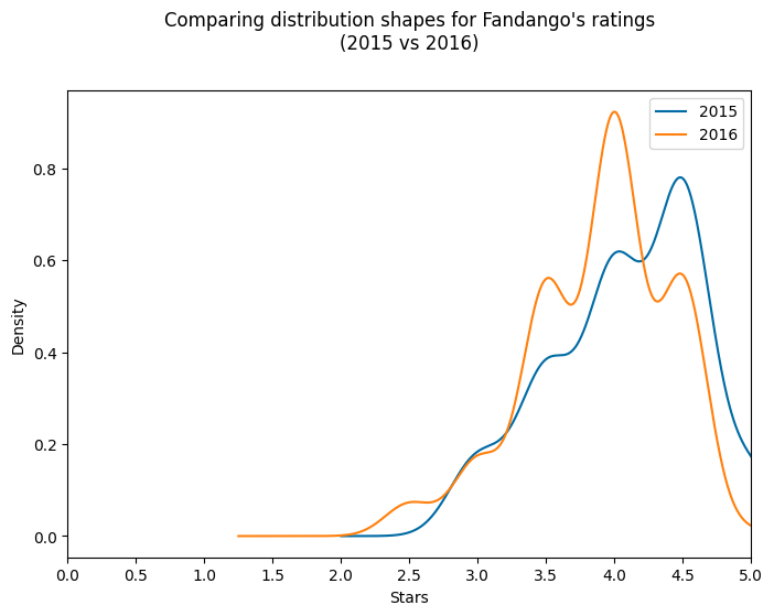
Once we analyze this visualization, we discover two attention-grabbing patterns:
- Each distributions are left-skewed, that means most scores are clustered towards the upper finish of the dimensions. This might counsel that Fandango typically offers favorable scores to motion pictures.
- The 2016 distribution seems to be barely shifted to the left in comparison with the 2015 distribution, indicating that scores may need been barely decrease in 2016.
Teacher Perception: I discover KDE plots a bit controversial for this type of information as a result of scores aren’t actually steady—they’re discrete values (complete or half stars). The dips you see within the KDE plot do not really exist within the information; they’re artifacts of the KDE algorithm attempting to bridge the gaps between discrete ranking values. Nonetheless, KDE plots are wonderful for shortly visualizing the general form and skew of distributions, which is why I am exhibiting them right here.
Let us take a look at the precise frequency of every ranking to get a extra correct image.
Step 6: Evaluating Relative Frequencies
To get a extra exact understanding of how the scores modified, let’s calculate the share of flicks that obtained every star ranking in each years:
print('2015 Scores Distribution')
print('-' * 25)
print(fandango_2015['Fandango_Stars'].value_counts(normalize=True).sort_index() * 100)

print('n2016 Scores Distribution')
print('-' * 25)
print(fandango_2016['fandango'].value_counts(normalize=True).sort_index() * 100)
The output reveals us the share breakdown of scores for every year:
2015 Scores Distribution
-------------------------
3.0     8.527132
3.5    17.829457
4.0    28.682171
4.5    37.984496
5.0     6.976744
Title: Fandango_Stars, dtype: float64

2016 Scores Distribution
-------------------------
2.5     3.141361
3.0     7.329843
3.5    24.083770
4.0    40.314136
4.5    24.607330
5.0     0.523560
Title: fandango, dtype: float64
Now, let’s remodel this right into a extra visually interesting bar chart of percentages to make the comparability simpler:
norm_2015 = fandango_2015['Fandango_Stars'].value_counts(normalize=True).sort_index() * 100
norm_2016 = fandango_2016['fandango'].value_counts(normalize=True).sort_index() * 100

df_freq = pd.DataFrame({
    '2015': norm_2015,
    '2016': norm_2016
})

df_freq.plot(variety='bar', figsize=(10, 6))
plt.title('Comparability of Fandango Ranking Distributions (2015 vs 2016)')
plt.xlabel('Star Ranking')
plt.ylabel('Proportion of Motion pictures')
plt.xticks(rotation=0)
plt.present()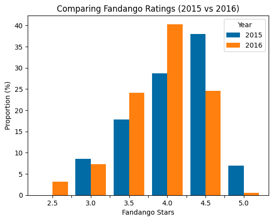
This visualization makes a number of patterns instantly clear:
- Excellent 5-star scores dropped dramatically: In 2015, almost 7% of flicks obtained an ideal 5-star ranking, however in 2016 this plummeted to simply 0.5%—a 93% lower!
- Very excessive 4.5-star scores additionally decreased: The share of flicks with 4.5 stars fell from about 38% in 2015 to simply beneath 25% in 2016.
- Center-high scores elevated: The share of flicks with 3.5 and 4.0 stars elevated considerably in 2016 in comparison with 2015.
- Decrease minimal ranking: The minimal ranking in 2016 was 2.5 stars, whereas in 2015 it was 3.0 stars.
These traits counsel that Fandango’s ranking system did certainly change between 2015 and 2016, with a shift towards barely decrease scores general.
Step 7: Calculating Abstract Statistics
To quantify the general change in scores, let’s calculate abstract statistics (imply, median, and mode) for each years:
mean_2015 = fandango_2015['Fandango_Stars'].imply()
mean_2016 = fandango_2016['fandango'].imply()

median_2015 = fandango_2015['Fandango_Stars'].median()
median_2016 = fandango_2016['fandango'].median()

mode_2015 = fandango_2015['Fandango_Stars'].mode()[0]
mode_2016 = fandango_2016['fandango'].mode()[0]

abstract = pd.DataFrame()
abstract['2015'] = [mean_2015, median_2015, mode_2015]
abstract['2016'] = [mean_2016, median_2016, mode_2016]
abstract.index = ['mean', 'median', 'mode']

abstract
This provides us:
       2015     2016
imply   4.085271 3.887435
median 4.000000 4.000000
mode   4.500000 4.000000
Let’s visualize these statistics to make the comparability clearer:
plt.model.use('fivethirtyeight')

abstract['2015'].plot.bar(coloration='#0066FF', align='heart', label='2015', width=.25)
abstract['2016'].plot.bar(coloration='#CC0000', align='edge', label='2016', width=.25, rot=0, figsize=(8, 5))

plt.title('Evaluating abstract statistics: 2015 vs 2016', y=1.07)
plt.ylim(0, 5.5)
plt.yticks(arange(0, 5.1, .5))
plt.ylabel('Stars')
plt.legend(framealpha=0, loc='higher heart')
plt.present()
If you run this code, you will produce the bar chart under evaluating the imply, median and mode for 2015 and 2016:
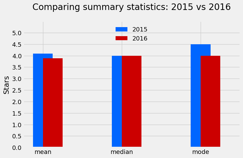
This visualization makes it instantly clear that scores had been typically decrease in 2016. It additionally confirms what we noticed within the distributions plot earlier:
- The imply ranking decreased from about 4.1 stars in 2015 to three.9 stars in 2016—a drop of about 5%.
- The median remained the identical at 4.0 stars for each years.
- The mode (most typical ranking) decreased from 4.5 stars in 2015 to 4.0 stars in 2016.
Teacher Perception: When presenting these findings to stakeholders, I would advocate the bar chart over the KDE plot. Whereas the KDE is nice for shortly understanding distribution shapes, the bar chart supplies extra correct illustration of the particular information with out introducing deceptive artifacts. The
framealpha=0parameter I used within the legend makes the legend background clear—it is a small styling element however makes the chart look extra skilled.
Step 8: Drawing Conclusions
Primarily based on our evaluation, we are able to confidently say that there was undoubtedly a change in Fandango’s ranking system between 2015 and 2016. The important thing findings embrace:
- General scores declined: The common film ranking dropped by about 0.2 stars (a 5% lower).
- Excellent scores almost disappeared: 5-star scores went from pretty widespread (7% of flicks) to extraordinarily uncommon (0.5% of flicks).
- Ranking inflation decreased: The proof means that Fandango’s tendency to inflate scores was decreased, with the distribution shifting towards extra reasonable (although nonetheless constructive) scores.
Whereas we won’t definitively show that these adjustments had been a direct response to Walt Hickey’s evaluation, the timing strongly means that Fandango did regulate their ranking system after being known as out for inflated scores. It seems that they addressed the problems Hickey recognized, significantly by eliminating the upward rounding that artificially boosted many scores.
Step 9: Limitations and Subsequent Steps
Our evaluation has a number of limitations to remember:
- Film high quality variation: We’re evaluating completely different units of flicks from completely different years. It is attainable (although unlikely) that 2016 motion pictures had been genuinely decrease high quality than 2015 motion pictures.
- Pattern representativeness: Each datasets had been collected utilizing non-random sampling strategies, which limits how confidently we are able to generalize our findings.
- Exterior elements: Adjustments in Fandango’s consumer base, reviewing insurance policies, or different exterior elements may have influenced the scores.
For additional evaluation, you may attempt answering these questions:
- Evaluating with different ranking platforms: Did related adjustments happen on IMDB, Rotten Tomatoes, or Metacritic throughout the identical interval?
- Analyzing by style: Had been sure kinds of motion pictures affected greater than others by the ranking system change?
- Extending the timeframe: How have Fandango’s scores developed in subsequent years?
- Investigating different ranking suppliers: Do different platforms that promote film tickets additionally present inflated scores?
Step 10: Sharing Your Challenge
Now that you have accomplished this evaluation, you may need to share it with others! Listed below are just a few methods to do this:
- GitHub Gist: For a fast and straightforward method to share your Jupyter Pocket book, you need to use GitHub Gist:
- Go to GitHub Gist
- Log in to your GitHub account (or create one if you do not have one)
- Click on on “New Gist”
- Copy and paste your Jupyter Pocket book code or add your .ipynb file
- Add an outline and choose “Create secret Gist” (non-public) or “Create public Gist” (seen to everybody)
- Portfolio web site: Add this undertaking to your information evaluation portfolio to showcase your expertise to potential employers.
- Dataquest Group: Share your evaluation within the Dataquest Group to get suggestions and have interaction with fellow learners.
Teacher Perception: GitHub Gists are considerably simpler to make use of than full Git repositories while you’re simply beginning out, and so they render Jupyter Notebooks fantastically. I nonetheless use them in the present day for fast sharing of notebooks with colleagues. For those who tag me within the Dataquest neighborhood (@Anna_Strahl), I would like to see your initiatives and supply suggestions!
Remaining Ideas
This undertaking demonstrates the facility of knowledge evaluation for investigating real-world questions on information integrity and bias. By utilizing comparatively easy instruments—information cleansing, visualization, and abstract statistics—we had been in a position to uncover significant adjustments in Fandango’s ranking system.
The investigation additionally reveals how public accountability by means of information journalism can drive corporations to handle points of their programs. After being uncovered for ranking inflation, Fandango seems to have made concrete adjustments to supply extra sincere scores to its customers.
For those who loved this undertaking and need to strengthen your information evaluation expertise additional, try different guided initiatives on Dataquest or attempt extending this evaluation with among the options within the “Subsequent Steps” part!
