
On this challenge walkthrough, we’ll discover the right way to section bank card clients utilizing unsupervised machine studying. By analyzing buyer conduct and demographic information, we’ll establish distinct buyer teams to assist a bank card firm develop focused advertising and marketing methods and enhance their backside line.
Buyer segmentation is a strong approach utilized by companies to grasp their clients higher. By grouping related clients collectively, corporations can tailor their advertising and marketing efforts, product choices, and customer support methods to fulfill the particular wants of every section, finally resulting in elevated buyer satisfaction and income.
On this tutorial, we’ll take you thru the entire machine studying workflow, from exploratory information evaluation to mannequin constructing and interpretation of outcomes.
What You may Study
By the tip of this tutorial, you may know the right way to:
- Carry out exploratory information evaluation on buyer information
- Remodel categorical variables for machine studying algorithms
- Use Ok-means clustering to section clients
- Apply the elbow methodology to find out the optimum variety of clusters
- Interpret and visualize clustering outcomes for actionable insights
Earlier than You Begin: Pre-Instruction
To profit from this challenge walkthrough, observe these preparatory steps:
- Evaluation the Venture
Entry the challenge and familiarize your self with the targets and construction: Buyer Segmentation Venture. - Put together Your Setting
- In the event you’re utilizing the Dataquest platform, all the things is already arrange for you.
- In the event you’re working regionally, guarantee you could have Python and Jupyter Pocket book put in, together with the required libraries:
pandas,numpy,matplotlib,seaborn, andsklearn. - To work on this challenge, you may want the
customer_segmentation.csvdataset, which accommodates details about the corporate’s purchasers, and we’re requested to assist section them into totally different teams with a purpose to apply totally different enterprise methods for every kind of buyer.
- Get Snug with Jupyter
- New to Markdown? We suggest studying the fundamentals to format headers and add context to your Jupyter pocket book: Markdown Information.
- For file sharing and challenge uploads, create a GitHub account.
Setting Up Your Setting
Earlier than we dive into creating our clustering mannequin, let’s overview the right way to use Jupyter Pocket book and arrange the required libraries for this challenge.
import pandas as pd
import numpy as np
import matplotlib.pyplot as plt
import seaborn as sns
from sklearn.preprocessing import StandardScaler
from sklearn.cluster import KMeans
Studying Perception: When working with scikit-learn, it’s normal apply to import particular capabilities or lessons fairly than all the library. This method retains your code clear and targeted, whereas additionally making it clear which instruments you are utilizing for every step of your evaluation.
Now let’s load our buyer information and take a primary take a look at what we’re working with:
df = pd.read_csv('customer_segmentation.csv')
df.head()| customer_id | age | gender | dependent_count | education_level | marital_status | estimated_income | months_on_book | total_relationship_count | months_inactive_12_mon | credit_limit | total_trans_amount | total_trans_count | avg_utilization_ratio |
|---|---|---|---|---|---|---|---|---|---|---|---|---|---|
| 768805383 | 45 | M | 3 | Excessive College | Married | 69000 | 39 | 5 | 1 | 12691.0 | 1144 | 42 | 0.061 |
| 818770008 | 49 | F | 5 | Graduate | Single | 24000 | 44 | 6 | 1 | 8256.0 | 1291 | 33 | 0.105 |
| 713982108 | 51 | M | 3 | Graduate | Married | 93000 | 36 | 4 | 1 | 3418.0 | 1887 | 20 | 0.000 |
| 769911858 | 40 | F | 4 | Excessive College | Unknown | 37000 | 34 | 3 | 4 | 3313.0 | 1171 | 20 | 0.760 |
| 709106358 | 40 | M | 3 | Uneducated | Married | 65000 | 21 | 5 | 1 | 4716.0 | 816 | 28 | 0.000 |
Understanding the Dataset
Let’s higher perceive our dataset by analyzing its construction and checking for lacking values:
df.information()
RangeIndex: 10127 entries, 0 to 10126
Information columns (whole 14 columns):
 #   Column                    Non-Null Rely  Dtype
---  ------                    --------------  -----
 0   customer_id               10127 non-null  int64
 1   age                       10127 non-null  int64
 2   gender                    10127 non-null  object
 3   dependent_count           10127 non-null  int64
 4   education_level           10127 non-null  object
 5   marital_status            10127 non-null  object
 6   estimated_income          10127 non-null  int64
 7   months_on_book            10127 non-null  int64
 8   total_relationship_count  10127 non-null  int64
 9   months_inactive_12_mon    10127 non-null  int64
 10  credit_limit              10127 non-null  float64
 11  total_trans_amount        10127 non-null  int64
 12  total_trans_count         10127 non-null  int64
 13  avg_utilization_ratio     10127 non-null  float64
dtypes: float64(2), int64(9), object(3)
reminiscence utilization: 1.1+ MB
Our dataset accommodates 10,127 buyer data with 14 variables. Luckily, there are not any lacking values, which simplifies our information preparation course of. Let’s perceive what every of those variables represents:
- customer_id: Distinctive identifier for every buyer
- age: Buyer’s age in years
- gender: Buyer’s gender (M/F)
- dependent_count: Variety of dependents (e.g., youngsters)
- education_level: Buyer’s schooling degree
- marital_status: Buyer’s marital standing
- estimated_income: Estimated annual revenue in {dollars}
- months_on_book: How lengthy the client has been with the bank card firm
- total_relationship_count: Variety of occasions the client has contacted the corporate
- months_inactive_12_mon: Variety of months the client did not use their card up to now 12 months
- credit_limit: Bank card restrict in {dollars}
- total_trans_amount: Complete quantity spent on the bank card
- total_trans_count: Complete variety of transactions
- avg_utilization_ratio: Common card utilization ratio (how a lot of their accessible credit score they use)
Earlier than we dive deeper into the evaluation, let’s examine the distribution of our categorical variables:
print(df['marital_status'].value_counts(), finish="nn")
print(df['gender'].value_counts(), finish="nn")
df['education_level'].value_counts()
marital_status
Married 4687
Single 3943
Unknown 749
Divorced 748
Title: rely, dtype: int64
gender
F 5358
M 4769
Title: rely, dtype: int64
education_level
Graduate 3685
Excessive College 2351
Uneducated 1755
Faculty 1192
Put up-Graduate 616
Doctorate 528
Title: rely, dtype: int64About half of the shoppers are married, adopted carefully by single clients, with smaller numbers of consumers with unknown marital standing or divorced.
The gender distribution is pretty balanced, with a slight majority of feminine clients (about 53%) in comparison with male clients (about 47%).
The schooling degree variable reveals that the majority clients have a graduate or highschool schooling, adopted by a considerable portion who’re uneducated. Smaller segments have attended school, achieved post-graduate levels, or earned a doctorate. This implies a variety of instructional backgrounds, with a majority concentrated in mid-level instructional attainment.
Exploratory Information Evaluation (EDA)
Now let’s discover the numerical variables in our dataset to grasp their distributions:
df.describe()This offers us a statistical abstract of our numerical variables, together with counts, means, normal deviations, and quantiles:
| customer_id | age | dependent_count | estimated_income | months_on_book | total_relationship_count | months_inactive_12_mon | credit_limit | total_trans_amount | total_trans_count | avg_utilization_ratio | |
|---|---|---|---|---|---|---|---|---|---|---|---|
| rely | 1.012700e+04 | 10127.000000 | 10127.000000 | 10127.000000 | 10127.000000 | 10127.000000 | 10127.000000 | 10127.000000 | 10127.000000 | 10127.000000 | 10127.000000 |
| imply | 7.391776e+08 | 46.325960 | 2.346203 | 62078.206774 | 35.928409 | 3.812580 | 2.341167 | 8631.953698 | 4404.086304 | 64.858695 | 0.274894 |
| std | 3.690378e+07 | 8.016814 | 1.298908 | 39372.861291 | 7.986416 | 1.554408 | 1.010622 | 9088.776650 | 3397.129254 | 23.472570 | 0.275691 |
| min | 7.080821e+08 | 26.000000 | 0.000000 | 20000.000000 | 13.000000 | 1.000000 | 0.000000 | 1438.300000 | 510.000000 | 10.000000 | 0.000000 |
| 25% | 7.130368e+08 | 41.000000 | 1.000000 | 32000.000000 | 31.000000 | 3.000000 | 2.000000 | 2555.000000 | 2155.500000 | 45.000000 | 0.023000 |
| 50% | 7.179264e+08 | 46.000000 | 2.000000 | 50000.000000 | 36.000000 | 4.000000 | 2.000000 | 4549.000000 | 3899.000000 | 67.000000 | 0.176000 |
| 75% | 7.731435e+08 | 52.000000 | 3.000000 | 80000.000000 | 40.000000 | 5.000000 | 3.000000 | 11067.500000 | 4741.000000 | 81.000000 | 0.503000 |
| max | 8.283431e+08 | 73.000000 | 5.000000 | 200000.000000 | 56.000000 | 6.000000 | 6.000000 | 34516.000000 | 18484.000000 | 139.000000 | 0.999000 |
To make it simpler to identify patterns, let’s visualize the distribution of every variable utilizing histograms:
fig, ax = plt.subplots(figsize=(12, 10))

# Eradicating the client's id earlier than plotting the distributions
df.drop('customer_id', axis=1).hist(ax=ax)

plt.tight_layout()
plt.present()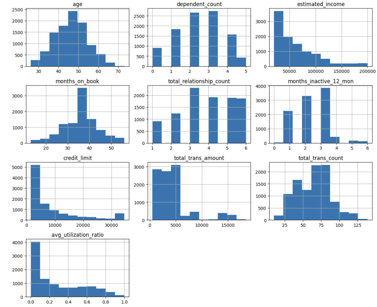
Studying Perception: When working with Jupyter and
matplotlib, you may see warning messages about a number of subplots. These are usually innocent and simply inform you thatmatplotlibis dealing with some facets of the plot creation routinely. For a portfolio challenge, you may need to refine your code to eradicate these warnings, however they do not have an effect on the performance or accuracy of your evaluation.
From these histograms, we will observe:
- Age: Pretty usually distributed, concentrated between 40-55 years
- Dependent Rely: Most clients have 0-3 dependents
- Estimated Earnings: Proper-skewed, with most clients having incomes beneath $100,000
- Months on E book: Usually distributed, centered round 36 months
- Complete Relationship Rely: Most clients have 3-5 contacts with the corporate
- Credit score Restrict: Proper-skewed, with most clients having a credit score restrict beneath $10,000
- Transaction Metrics: Each quantity and rely present some proper skew
- Utilization Ratio: Many shoppers have very low utilization (close to 0), with a smaller group having excessive utilization
Subsequent, let’s take a look at correlations between variables to grasp relationships inside our information and visualize them utilizing a heatmap:
correlations = df.drop('customer_id', axis=1).corr(numeric_only=True)

fig, ax = plt.subplots(figsize=(12,8))
sns.heatmap(correlations[(correlations > 0.30) | (correlations < -0.30)],
            cmap='Blues', annot=True, ax=ax)

plt.tight_layout()
plt.present()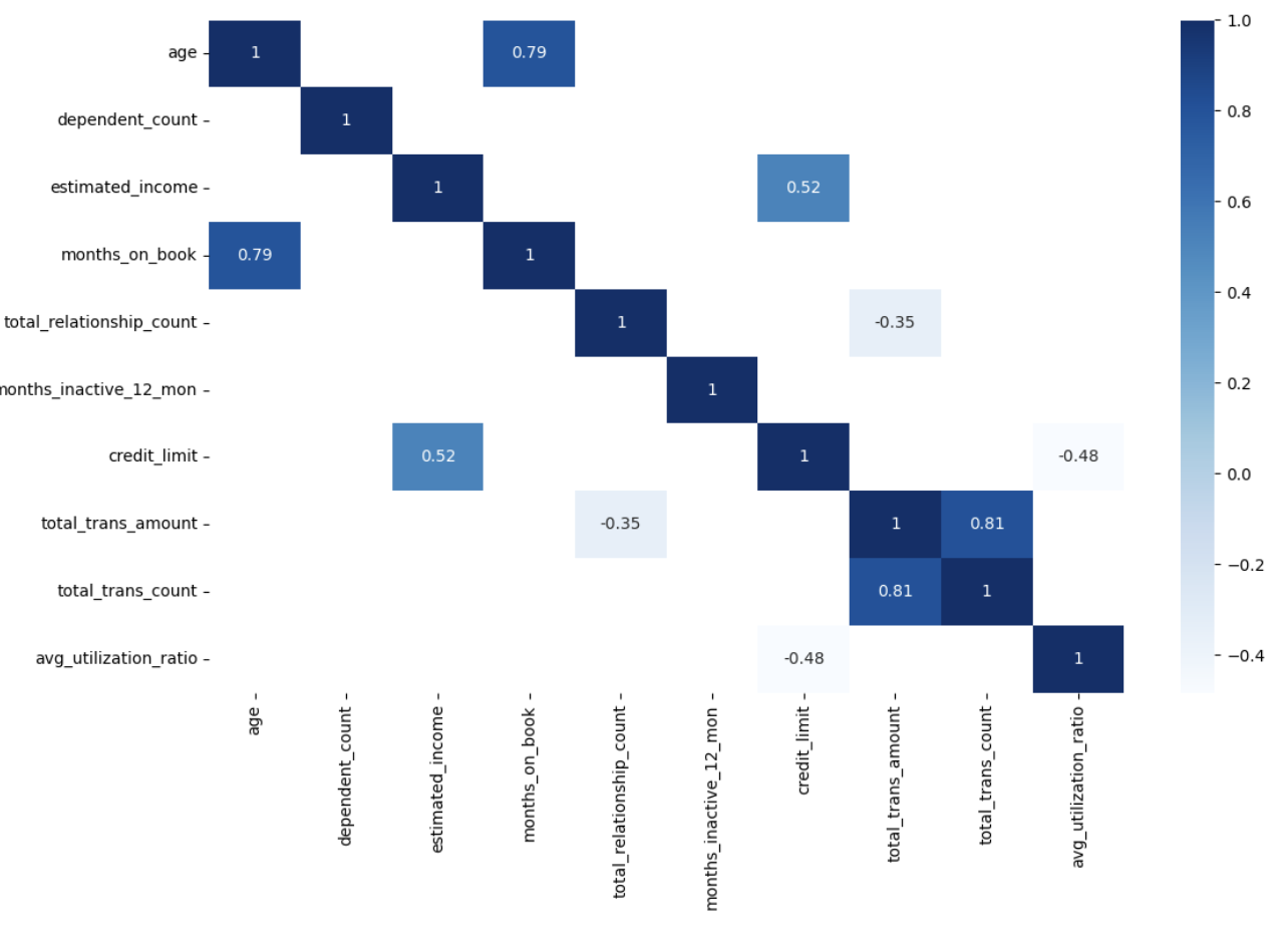
Studying Perception: When creating correlation heatmaps, filtering to indicate solely stronger correlations (e.g., these above 0.3 or beneath -0.3) could make the visualization rather more readable and aid you concentrate on a very powerful relationships in your information.
The correlation heatmap reveals a number of fascinating relationships:
- Age and Months on E book: Robust optimistic correlation (0.79), suggesting older clients have been with the corporate longer
- Credit score Restrict and Estimated Earnings: Constructive correlation (0.52), which is sensible as greater revenue sometimes qualifies for greater credit score limits
- Transaction Quantity and Rely: Robust optimistic correlation (0.81), which means clients who make extra transactions additionally spend extra total
- Credit score Restrict and Utilization Ratio: Detrimental correlation (-0.48), suggesting clients with greater credit score limits have a tendency to make use of a smaller proportion of their accessible credit score
- Relationship Rely and Transaction Quantity: Detrimental correlation (-0.35), curiously indicating that clients who contact the corporate extra are inclined to spend much less
These relationships shall be precious to contemplate as we interpret our clustering outcomes later.
Characteristic Engineering
Earlier than we will apply Ok-means clustering, we have to remodel our categorical variables into numerical representations. Ok-means operates by calculating distances between factors in a multi-dimensional area, so all options should be numeric.
Let’s deal with every categorical variable appropriately:
1. Gender Transformation
Since gender is binary on this dataset (M/F), we will use a easy mapping:
customers_modif = df.copy()

customers_modif['gender'] = df['gender'].apply(lambda x: 1 if x == 'M' else 0)
customers_modif.head()
Studying Perception: When a categorical variable has solely two classes, you need to use a easy binary encoding (0/1) fairly than one-hot encoding. This reduces the dimensionality of your information and might result in extra interpretable fashions.
2. Training Degree Transformation
Training degree has a pure ordering (uneducated < highschool < school, and many others.), so we will use ordinal encoding:
education_mapping = {'Uneducated': 0, 'Excessive College': 1, 'Faculty': 2,
                     'Graduate': 3, 'Put up-Graduate': 4, 'Doctorate': 5}
customers_modif['education_level'] = customers_modif['education_level'].map(education_mapping)

customers_modif.head()
3. Marital Standing Transformation
Marital standing would not have a pure ordering, and it has greater than two classes, so we’ll use one-hot encoding:
dummies = pd.get_dummies(customers_modif[['marital_status']])

customers_modif = pd.concat([customers_modif, dummies], axis=1)
customers_modif.drop(['marital_status'], axis=1, inplace=True)

print(customers_modif.information())
customers_modif.head()
RangeIndex: 10127 entries, 0 to 10126
Information columns (whole 17 columns):
 #   Column                    Non-Null Rely  Dtype
---  ------                    --------------  -----
 0   customer_id               10127 non-null  int64
 1   age                       10127 non-null  int64
 2   gender                    10127 non-null  int64
 3   dependent_count           10127 non-null  int64
 4   education_level           10127 non-null  int64
 5   estimated_income          10127 non-null  int64
 6   months_on_book            10127 non-null  int64
 7   total_relationship_count  10127 non-null  int64
 8   months_inactive_12_mon    10127 non-null  int64
 9   credit_limit              10127 non-null  float64
 10  total_trans_amount        10127 non-null  int64
 11  total_trans_count         10127 non-null  int64
 12  avg_utilization_ratio     10127 non-null  float64
 13  marital_status_Divorced   10127 non-null  bool
 14  marital_status_Married    10127 non-null  bool
 15  marital_status_Single     10127 non-null  bool
 16  marital_status_Unknown    10127 non-null  bool
dtypes: bool(4), float64(2), int64(11)
reminiscence utilization: 1.0 MB
Studying Perception: One-hot encoding creates a brand new binary column for every class, which might result in an “implicit weighting” impact if a variable has many classes. That is one thing to pay attention to when decoding clustering outcomes, as it could actually generally trigger the algorithm to prioritize variables with extra classes.
Now our information is absolutely numeric and prepared for scaling and clustering.
Scaling the Information
Ok-means clustering makes use of distance-based calculations, so it is necessary to scale our options to make sure that variables with bigger ranges (like revenue) do not dominate the clustering course of over variables with smaller ranges (like age).
X = customers_modif.drop('customer_id', axis=1)

scaler = StandardScaler()
scaler.match(X)

X_scaled = scaler.remodel(X)
Studying Perception:
StandardScalertransforms every characteristic to have a imply of 0 and a normal deviation of 1. This places all options on an equal footing, no matter their unique scales. For Ok-means clustering, that is what ensures that every characteristic contributes equally to the space calculations.
Discovering the Optimum Variety of Clusters
One of many challenges with Ok-means clustering is figuring out the optimum variety of clusters. The elbow methodology is a standard method, the place we plot the sum of squared distances (inertia) for various numbers of clusters and search for an “elbow” level the place the speed of lower sharply modifications.
X = pd.DataFrame(X_scaled)
inertias = []

for okay in vary(1, 11):
    mannequin = KMeans(n_clusters=okay)
    y = mannequin.fit_predict(X)
    inertias.append(mannequin.inertia_)

plt.determine(figsize=(12, 8))
plt.plot(vary(1, 11), inertias, marker='o')
plt.xticks(ticks=vary(1, 11), labels=vary(1, 11))
plt.title('Inertia vs Variety of Clusters')

plt.tight_layout()
plt.present()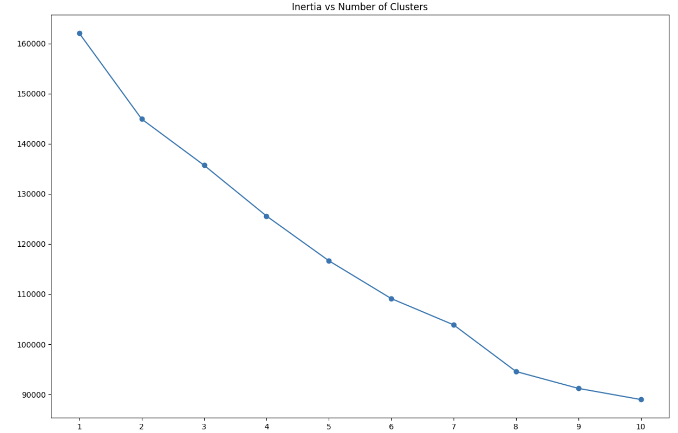
Studying Perception: The elbow methodology is not all the time crystal clear, and there is typically some judgment concerned in choosing the “proper” variety of clusters. Think about working the clustering a number of occasions with totally different numbers of clusters and evaluating which answer supplies probably the most actionable insights for your corporation context.
In our case, the plot means that round 5-8 clusters could possibly be acceptable, because the lower in inertia begins to degree off on this vary. For this evaluation, we’ll select 8 clusters, because it seems to strike a great stability between element and interpretability.
Constructing the Ok-Means Clustering Mannequin
Now that we have decided the optimum variety of clusters, let’s construct our Ok-means mannequin:
mannequin = KMeans(n_clusters=8)
y = mannequin.fit_predict(X_scaled)

# Including the cluster assignments to our unique dataframe
df['CLUSTER'] = y + 1  # Including 1 to make clusters 1-based as a substitute of 0-based
df.head()
Let’s examine what number of clients we have now in every cluster:
df['CLUSTER'].value_counts()CLUSTER
5 2015
7 1910
2 1577
1 1320
4 1045
6 794
3 736
8 730
Title: rely, dtype: int64Our clusters have moderately balanced sizes, with no single cluster dominating the others.
Analyzing the Clusters
Now that we have created our buyer segments, let’s analyze them to grasp what makes every cluster distinctive. We’ll begin by analyzing the typical values of numeric variables for every cluster:
numeric_columns = df.select_dtypes(embrace=np.quantity).drop(['customer_id', 'CLUSTER'], axis=1).columns

fig = plt.determine(figsize=(20, 20))
for i, column in enumerate(numeric_columns):
    df_plot = df.groupby('CLUSTER')[column].imply()
    ax = fig.add_subplot(5, 2, i+1)
    ax.bar(df_plot.index, df_plot, colour=sns.color_palette('Set1'), alpha=0.6)
    ax.set_title(f'Common {column.title()} per Cluster', alpha=0.5)
    ax.xaxis.grid(False)

plt.tight_layout()
plt.present()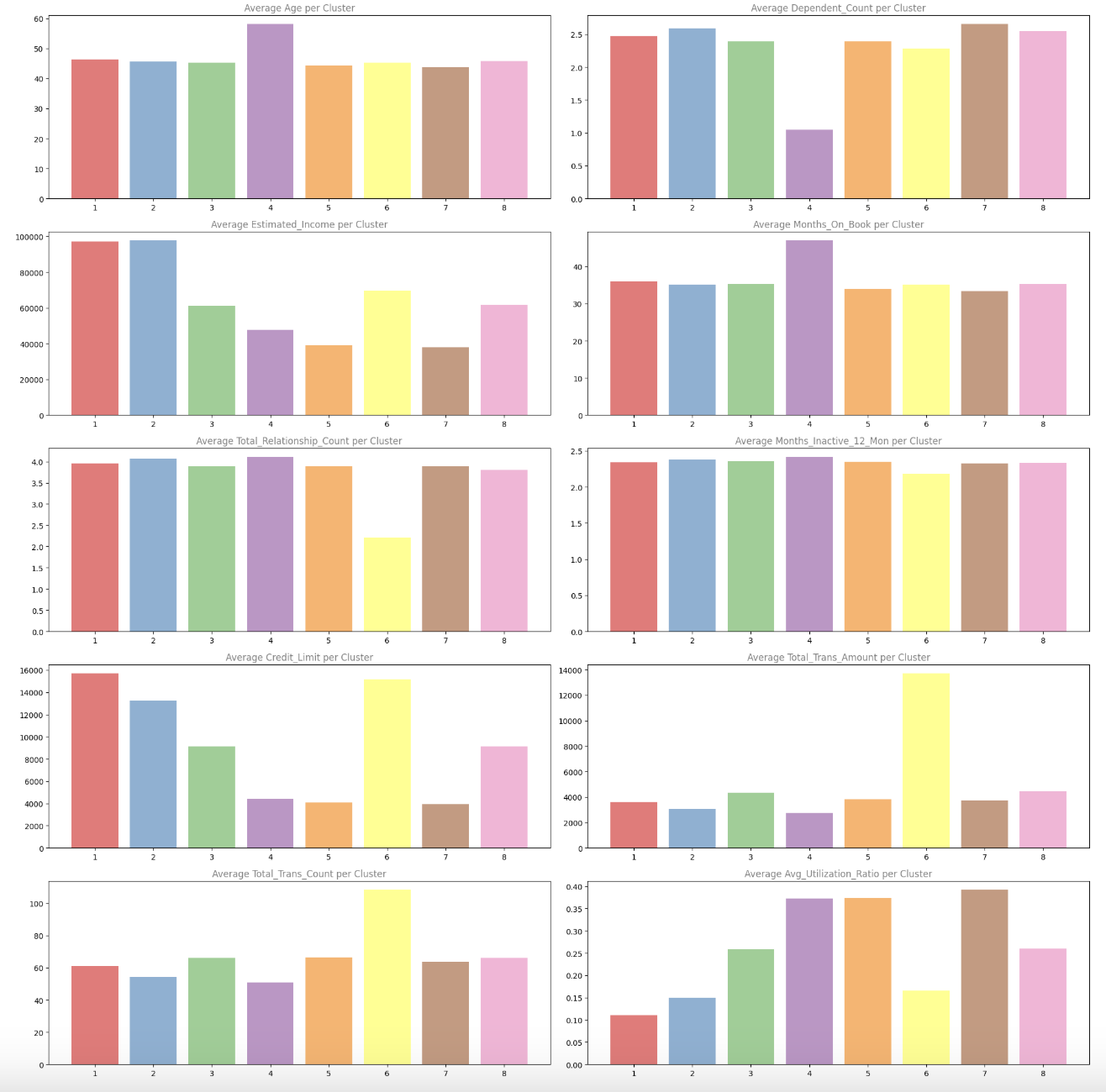
These bar charts assist us perceive how every variable differs throughout clusters. For instance, we will see:
- Estimated Earnings: Clusters 1 and a pair of have considerably greater common incomes
- Credit score Restrict: Equally, Clusters 1 and a pair of have greater credit score limits
- Transaction Metrics: Cluster 6 stands out with a lot greater transaction quantities and counts
Let’s additionally take a look at how the clusters seem in scatter plots of key variables:
fig, ((ax1, ax2), (ax3, ax4)) = plt.subplots(2, 2, figsize=(16, 8))
sns.scatterplot(x='age', y='months_on_book', hue='CLUSTER', information=df, palette='tab10', alpha=0.4, ax=ax1)
sns.scatterplot(x='estimated_income', y='credit_limit', hue='CLUSTER', information=df, palette='tab10', alpha=0.4, ax=ax2, legend=False)
sns.scatterplot(x='credit_limit', y='avg_utilization_ratio', hue='CLUSTER', information=df, palette='tab10', alpha=0.4, ax=ax3)
sns.scatterplot(x='total_trans_count', y='total_trans_amount', hue='CLUSTER', information=df, palette='tab10', alpha=0.4, ax=ax4, legend=False)

plt.tight_layout()
plt.present()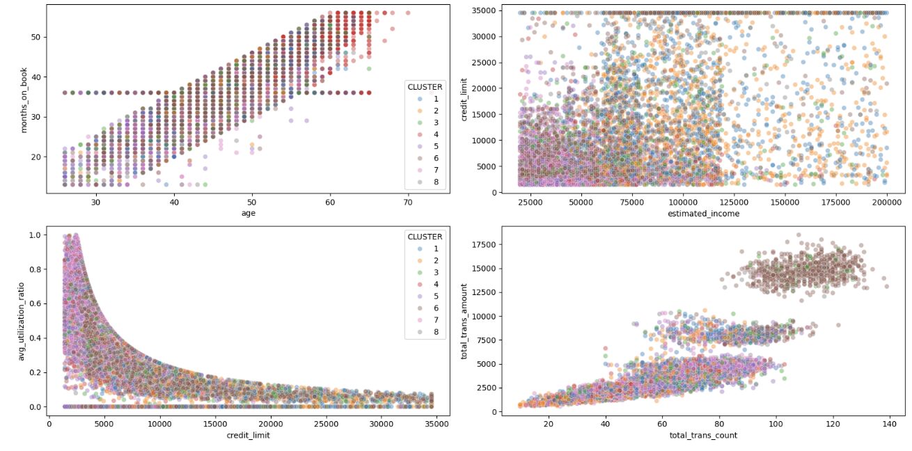
The scatter plots reveal some fascinating patterns:
- Within the Credit score Restrict vs. Utilization Ratio plot, we will see distinct clusters with totally different behaviors – some have excessive credit score limits however low utilization, whereas others have decrease limits however greater utilization
- The Transaction Rely vs. Quantity plot reveals Cluster 6 as a definite group with excessive transaction exercise
- The Age vs. Months on E book plot reveals the anticipated optimistic correlation, however with some fascinating cluster separations
Lastly, let’s look at the distribution of categorical variables throughout clusters:
cat_columns = df.select_dtypes(embrace=['object'])

fig = plt.determine(figsize=(18, 6))
for i, col in enumerate(cat_columns):
    plot_df = pd.crosstab(index=df['CLUSTER'], columns=df[col], values=df[col], aggfunc='measurement', normalize='index')
    ax = fig.add_subplot(1, 3, i+1)
    plot_df.plot.bar(stacked=True, ax=ax, alpha=0.6)
    ax.set_title(f'% {col.title()} per Cluster', alpha=0.5)

    ax.set_ylim(0, 1.4)
    ax.legend(frameon=False)
    ax.xaxis.grid(False)

plt.tight_layout()
plt.present()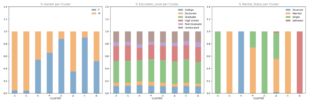
These stacked bar charts reveal some robust patterns:
- Gender: Some clusters are closely skewed in direction of one gender (e.g., Clusters 5 and seven are predominantly feminine)
- Marital Standing: Sure clusters are strongly related to particular marital statuses (e.g., Cluster 2 is generally married, Cluster 5 is generally single)
- Training Degree: This reveals extra blended patterns throughout clusters
Studying Perception: The robust affect of marital standing on our clustering outcomes could be partly as a result of one-hot encoding we used, which created 4 separate columns for this variable. In future iterations, you may need to experiment with totally different encoding strategies or scaling to see the way it impacts your outcomes.
Buyer Phase Profiles
Based mostly on our evaluation, we will create profiles for every buyer section, summarized within the desk beneath:
| Excessive-Earnings Single Males | • Predominantly male • Principally single |
• Excessive revenue (~$100K) • Excessive credit score restrict |
• Low bank card utilization (10%) | These clients have cash to spend however aren’t utilizing their playing cards a lot. The corporate may provide rewards or incentives particularly tailor-made to single professionals to encourage extra card utilization. | |
| Prosperous Household Males | • Predominantly male • Married • Greater variety of dependents (~2.5) |
• Excessive revenue (~$100K) • Excessive credit score restrict |
• Low utilization ratio (15%) | These clients symbolize family-oriented excessive earners. Household-focused rewards applications or partnerships with family-friendly retailers may enhance their card utilization. | |
| Divorced Mid-Earnings Clients | • Combined gender • Predominantly divorced |
• Common revenue and credit score restrict | • Common transaction patterns | This section may reply nicely to monetary planning providers or stability-focused messaging as they navigate post-divorce funds. | |
| Older Loyal Clients | • 60% feminine • 70% married • Oldest common age (~60) |
• Decrease credit score restrict • Greater utilization ratio |
• Longest relationship with the corporate • Few dependents |
These loyal clients may admire recognition applications and senior-focused advantages. | |
| Younger Single Ladies | • 90% feminine • Predominantly single |
• Lowest common revenue (~$40K) • Low credit score restrict |
• Excessive utilization ratio | This section may profit from entry-level monetary schooling and accountable credit score utilization applications. They could even be receptive to credit score restrict enhance provides as their careers progress. | |
| Massive Spenders | • 60% male • Mixture of single and married |
• Above-average revenue (~$70K) • Excessive credit score restrict |
• Highest transaction rely and quantity by a big margin | These are the corporate’s most lively clients. Premium rewards applications and unique perks may assist preserve their excessive engagement. | |
| Household-Targeted Ladies | • 90% feminine • Married • Highest variety of dependents |
• Low revenue (~$40K) • Low credit score restrict paired with excessive utilization |
• Average transaction patterns | This section may reply nicely to family-oriented promotions and cash-back on on a regular basis purchases like groceries and youngsters’s gadgets. | |
| Unknown Marital Standing | • Combined gender • All with unknown marital standing |
• Common throughout most metrics | • No distinct patterns | This section primarily exists attributable to lacking information. The corporate ought to try and replace these data to raised categorize these clients. |
Challenges and Concerns
Our evaluation revealed some fascinating patterns, but in addition highlighted a possible concern with our method. The robust affect of marital standing on our clustering outcomes means that our one-hot encoding of this variable may need given it extra weight than supposed. This “implicit weighting” impact is a standard problem when utilizing one-hot encoding with Ok-means clustering.
For future iterations, we’d contemplate:
- Various Encoding Strategies: Attempt totally different approaches for categorical variables
- Take away Particular Classes: Take a look at if eradicating the “Unknown” marital standing modifications the clustering patterns
- Totally different Distance Metrics: Experiment with different distance calculations for Ok-means
- Characteristic Choice: Explicitly select which options to incorporate within the clustering
Abstract of Evaluation
On this challenge, we have demonstrated how unsupervised machine studying can be utilized to section clients primarily based on their demographic and behavioral traits. These segments present precious insights {that a} bank card firm can use to develop focused advertising and marketing methods and enhance buyer engagement.
Our evaluation recognized eight distinct buyer segments, every with their very own traits and alternatives for focused advertising and marketing:
- Excessive-income single males
- Prosperous household males
- Divorced mid-income clients
- Older loyal clients
- Younger single girls
- Massive spenders
- Household-focused girls
- Unknown marital standing (potential information concern)
These groupings may also help the corporate tailor their advertising and marketing messages, rewards applications, and product choices to the particular wants and behaviors of every buyer section, doubtlessly resulting in elevated card utilization, buyer satisfaction, and income.
Subsequent Steps
To take this evaluation additional, you may attempt your hand at these enhancements:
- Validate the Clusters: Use silhouette scores or different metrics to quantitatively consider the standard of the clusters
- Experiment with Totally different Algorithms: Attempt hierarchical clustering or DBSCAN as alternate options to Ok-means
- Embrace Extra Information: Incorporate extra buyer variables, resembling spending classes or fee behaviors
- Temporal Evaluation: Analyze how clients transfer between segments over time
We have now another challenge walkthrough tutorials you may additionally get pleasure from:
In the event you’re new to Python and don’t really feel prepared to begin this challenge, start with our Python Fundamentals for Information Evaluation ability path to construct the foundational expertise wanted for this challenge. The course covers important subjects like loops, conditionals, and information manipulation with pandas that we have used extensively on this evaluation. When you’re snug with these ideas, come again to construct your personal buyer segmentation mannequin and tackle the enhancement challenges!
Completely happy coding!

